Normalize lag times across files
![]()
dyco uses eddy covariance raw data files as input and produces lag-compensated raw data files as output.
Version 2 changes the previous workflow.
dyco identifies and corrects time lags between variables. It iteratively searches for lags between two variables,
e.g., W (turbulent vertical wind) and S (scalar used for time lag detection, e.g. CO2 or CH4),
starting with a broad time window and progressively narrowing it based on the distribution of found lags. This iterative
refinement helps pinpoint consistent lags, suggesting strong covariance. Lag searches can be performed on short segments
of a long file. After collecting all identified lags, dyco filters outliers and creates a look-up table of daily time
lags. This table is then used to shift variables in the input files, correcting for the identified lags. While S is
typically used for lag detection, the correction can be applied to other variables as needed. Lags are expressed in “
number of records”; the corresponding time depends on the data’s recording frequency.
v2Generally, dyco v2 follows the workflow:
dyco detects the time lag between two variables, e.g. W and S. It begins by searching for this lag within a broad
time window, for
example, e.g. between -1000 and +1000 data points ([-1000, 1000]). This initial search is considered
iteration 1.
Lag is always expressed as “number of records”. If the underlying data were recorded at 20Hz, then 1000 records
correspond to 50 seconds of measurements. Negative time lags mean that S lags behind W by the respective number of
records.
Lag search can be done in segments per file. For example, for a file with 30 minutes of data, the lag can be
detected in three 10-minute segments, yielding three detected time lags for the respective file. Another example, for a
file with 24 hours of data, the lag can be detected for 30-minute segments, yielding 48 time lags.

Figure 1. Results from the covariance calculation (iteration 1) between turbulent vertical wind and turbulent CH4
mixing ratios from the subcanopy station CH-DAS on
17 May 2023. Time lag was searched between -500 and 0 records in a 10MIN segment between 10:20 and 10:30, extracted
from a 30MIN data file. Peak absolute covariance was found at lag -246, which means that S (CH4) arrived 246 records
after W (vertical wind) at the sensor.
Next, dyco analyzes the distribution of the identified time lags. It identifies the most frequent lag (the peak of the
histogram, e.g., -220) and creates a smaller search window around it. For example, a new window like [-758, +196]
might be defined. This narrowing process expands outward from the peak lag until a certain percentage of the data (e.g.,
95%) is encompassed within the new window.

Figure 2. Histogram of found time lags (iteration 1) between turbulent vertical wind and turbulent CH4 mixing
ratios using a search window of [-500, 0] records. This example used 6919 data files between 12 May 2023 and 31 Dec
2023, recorded at 30MIN time resolution. The lag was detected in 10MIN segments for each file, i.e., covariance
calculations for each 30MIN file yielded 3 time lags (6919 * 3 = 20757 time lags, the figure shows only 20373 because
for some files no time lag could be calculated, e.g. due to few records). A clear peak distribution just below -200
indicates a range where lags were found consistently. Based on these results, the window size for the next iteration is
set. Here, the window size for the next iteration was set to -485 (blue dashed line) and -5 (not visible because close
to the lag zero line).
The second iteration repeats the lag search process in Step 1 and the lag analysis in Step 2, but now using the refined,
narrower time window from the previous step. This process can be repeated multiple times, there is no limit for the
number of iterations. However, it’s important to monitor the size of the time window in each iteration to ensure it
remains sufficiently large for accurate results.
Across all iterations, all time lags found for S are collected. Time lags found for a specific file can appear
multiple times in the collected results, depending on the number of iterations. This helps in identifying time lags that
remain constant despite the continuously narrower time windows for lag search, indicating potentially high covariance
between W and S.
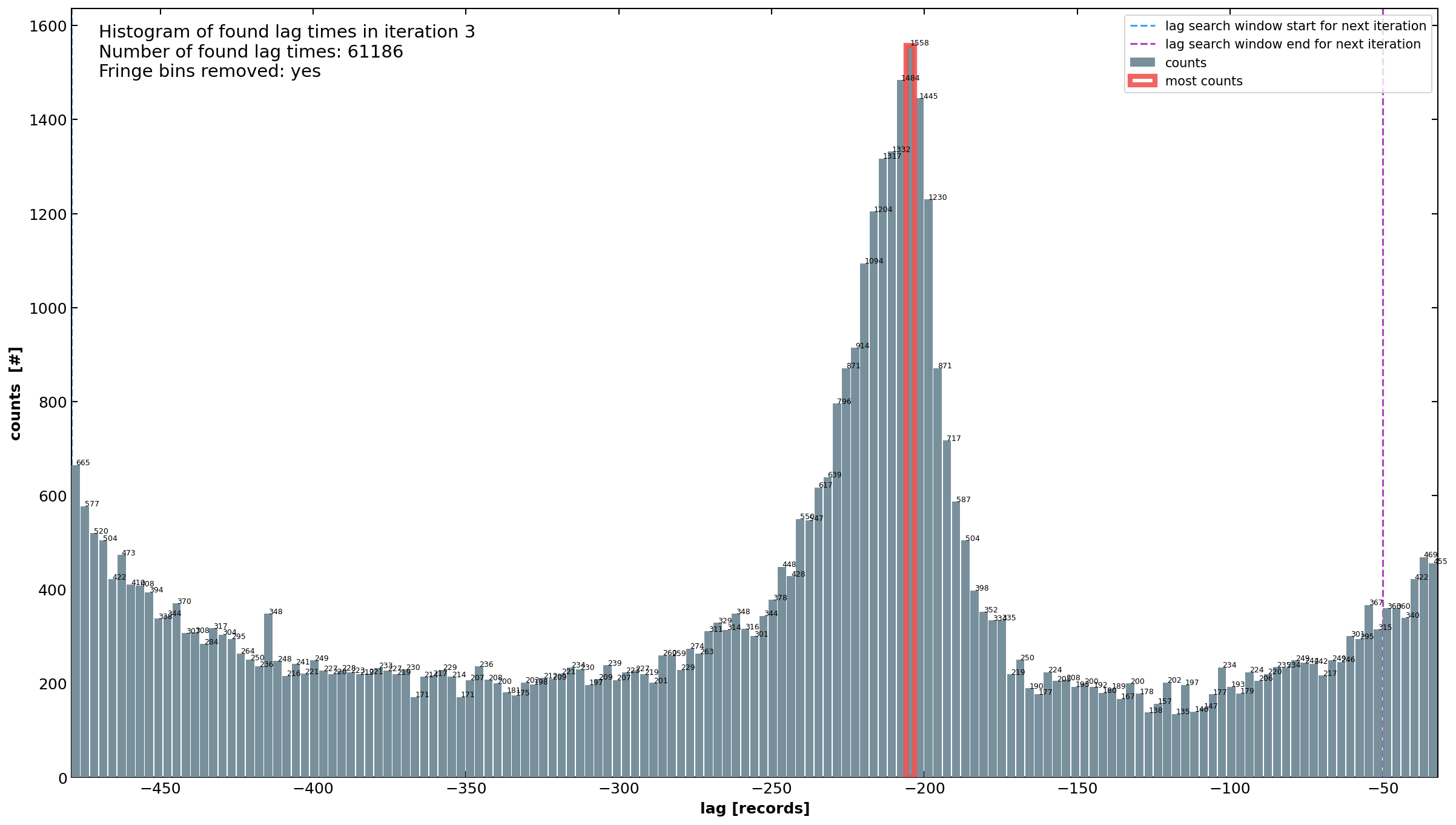
Figure 3. Histogram displaying the distribution of identified time lags after the third iteration within a narrowed
time window of [-482, -26] records. Minimal window shortening was needed in previous iterations as the initial range
of [-500, 0] was well-suited. Note the number of found lag times: this number also includes lags from all previous
iterations.
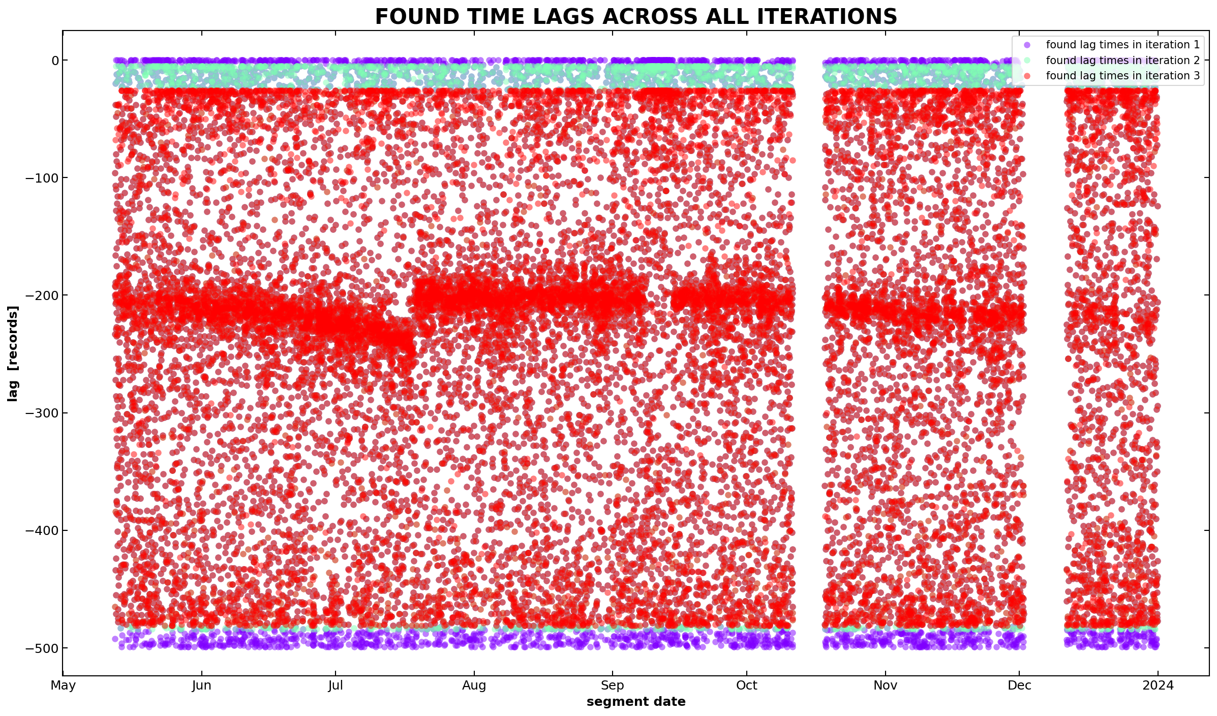
Figure 4. Time series plot of all found time lags across all files and iterations. An accumulation of found time
lags around lag -200 is clearly visible. The time lags are not constant but show a clear drift.
After collecting all time lags across all iterations, dyco analyzes these results. It uses a Hampel filter to remove
outliers, ensuring that only consistent and similar lags are retained.
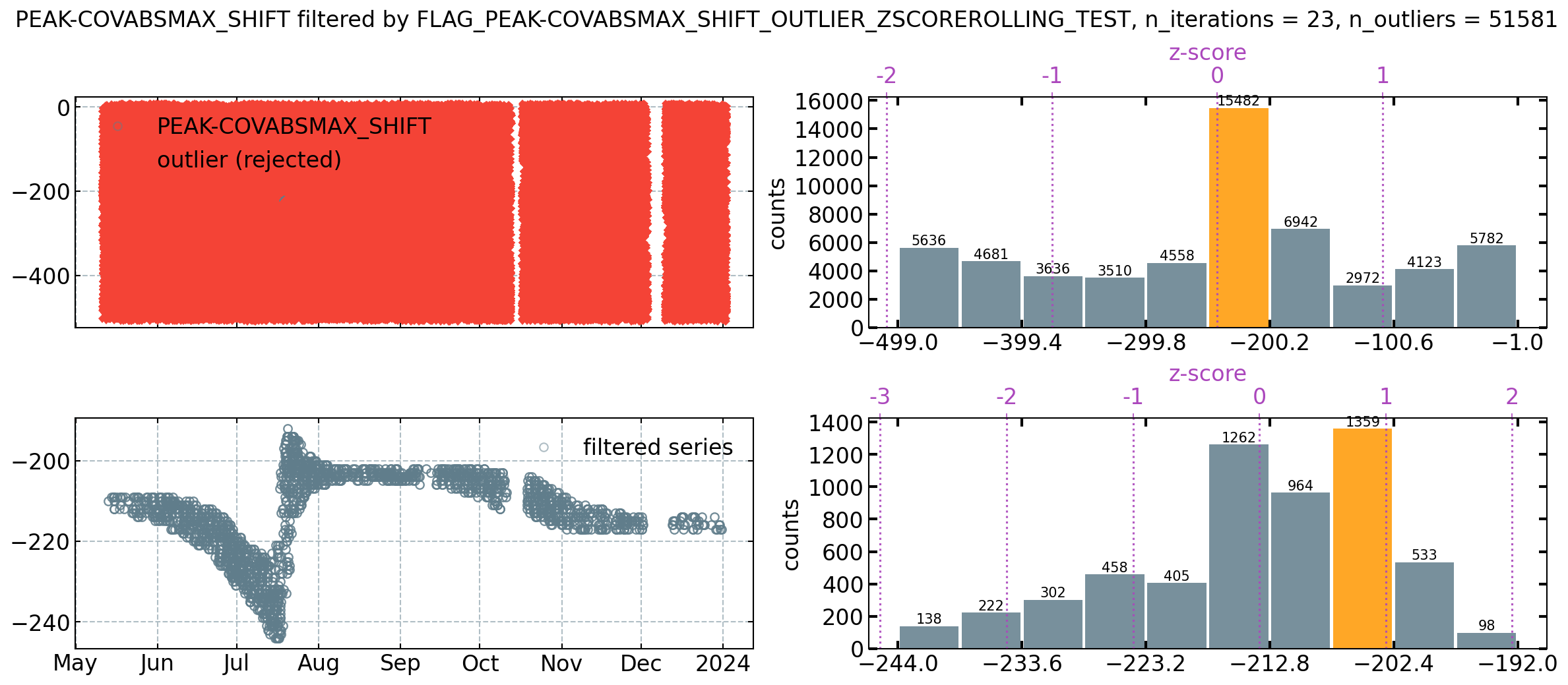
Figure 5. Application of a Hampel filter for outlier removal to retain consistent and similar lags. The lower left
panel shows found time lags after outlier removal. These lags are used to create a look-up table.
The outlier-filtered time lags are used to create a look-up table, providing time lag information for each day.
The generated look-up table is then used to adjust the input data files. For each file, the corresponding time lag from
the table is applied to shift one or more variables. While S is used for lag detection, the lag correction can be
applied to S itself or to other variables of interest. This flexibility allows dyco to leverage a strong S signal
for lag detection even if S itself is not the primary target for lag correction.

Figure 6. Time series of found time lags across all iterations and files. The 5-day median was calculated from
found high-quality time lags (when cross-covariance analyses yielded a clear covariance peak) after outlier removal and
is used to shift each scalar of interest (e.g., CH4) in each data file by the respective number of records. The 5-day
median is calculated at the daily scale, i.e., data files from a specific day are shifted by the same amount of records.
After this lag compensation, the time lags between wind and scalar(s) is at or close to zero.
Results from all steps are stored to output folders in a specified output directory.
After the lag was removed from the scalars of interest, the data files can be directly used for flux calculations.
The lag detection between the turbulent departures of measured wind and the scalar of interest is a central step in the
calculation of eddy covariance (EC) ecosystem fluxes. In case the covariance maximization fails to detect a clear peak
in the covariance function between the wind and the scalar, current flux calculation software can apply a constant
default (nominal) time lag to the respective scalar. However, both the detection of clear covariance peaks in a
pre-defined time window and the definition of a reliable default time lag is challenging for compounds which are often
characterized by low SNR (signal-to-noise ratio), such as N2O. In addition, the application of one static
default time lag may produce inaccurate results in case systematic time shifts are present in the raw data.
dyco is meant to assist current flux processing software in the calculation of fluxes for compounds with low SNR. In
the context of current flux processing schemes, the unique features offered as part of the dyco package include:
As dyco aims to complement current flux processing schemes, final lag-removed files are produced that can be directly
used in current flux calculation software.
In ecosystem research, the EC method is widely used to quantify the biosphere-atmosphere exchange of greenhouse gases (
GHGs) and energy (Aubinet et al., 2012; Baldocchi et al., 1988). The raw ecosystem flux (i.e. net exchange) is
calculated by the covariance between the turbulent vertical wind component measured by a sonic anemometer and the entity
of interest, e.g. CO2, measured by a gas analyzer. Due to the application of two different instruments, wind
and gas are not recorded at exactly the same time, resulting in a time lag between the two time series. For the
calculation of ecosystem fluxes this time delay has to be quantified and corrected for, otherwise fluxes are
systematically biased. Time lags for each averaging interval can be estimated by finding the maximum absolute covariance
between the two turbulent time series at different time steps in a pre-defined time window of physically possible
time-lags (e.g., McMillen, 1988; Moncrieff et al., 1997). Lag detection works well when processing fluxes for compounds
with high signal-to-noise ratio (SNR), which is typically the case for e.g. CO2. In contrast, for compounds
with low SNR (e.g., N2O, CH4) the cross-covariance function with the turbulent wind component
yields noisier results and calculated fluxes are biased towards larger absolute flux values (Langford et al., 2015),
which in turn renders the accurate calculation of yearly ecosystem GHG budgets more difficult and results may be
inaccurate.
One suggestion to adequately calculate fluxes for compounds with low SNR is to first calculate the time lag for a
reference compound with high SNR (e.g. CO2) and then apply the same time lag to the target compound of
interest (e.g. N2O), with both compounds being recorded by the same analyzer (Nemitz et al., 2018). dyco
follows up on this suggestion by facilitating the dynamic lag-detection between the turbulent wind data and a
reference compound and the subsequent application of found reference time lags to one or more target compounds.
dyco can be installed via pip:
pip install dyco
Currently dyco needs input files where the vertical wind component and the scalars of interest were already rotated (
2D wind rotation to obtain turbulent departures for wind and scalars). In the example below this rotation was done using
the class FileSplitterMulti from the Python library diive. This class can split
longer files into shorter files and rotate variables in the same step.
The class Dyco can be used in code. See class docstring for more details.
from dyco.dyco import DycoDyco(var_reference="W_[R350-B]_TURB", # Turbulent departures of the vertical wind component from the sonic anemometervar_lagged="CH4_DRY_[QCL-C2]_TURB", # Turbulent departures of the CH4 mixing ratiovar_target=["CH4_DRY_[QCL-C2]_TURB", "N2O_DRY_[QCL-C2]_TURB"],indir=r"F:\example\input_files",outdir=r"F:\example\output",filename_date_format="CH-DAS_%Y%m%d%H%M%S_30MIN-SPLIT_ROT_TRIM.csv",filename_pattern="CH-DAS_*_30MIN-SPLIT_ROT_TRIM.csv",files_how_many=None,file_generation_res="30min",file_duration="30min",data_timestamp_format="%Y-%m-%d %H:%M:%S.%f",data_nominal_timeres=0.05,lag_segment_dur="10min",lag_winsize=1000,lag_n_iter=3,lag_hist_remove_fringe_bins=True,lag_hist_perc_thres=0.7,target_lag=0,del_previous_results=False)
dyco can be run from the command line interface (CLI).
usage: dyco.py [-h]var_referenceColumn name of the unlagged reference variable in the data files (one-row header).Lags are determined in relation to this signal.var_laggedColumn name of the lagged variable in the data files (one-row header).The time lag of this signal is determined in relation to the reference signal var_reference.var_target [var_target2, var_target3 ...]Column name(s) of the target variable(s). Column names of the variables the lag that wasfound between var_reference and var_lagged should be applied to. Example: var1 var2 var3[-i INDIR]Path to the source folder that contains the data files, e.g. C:/dyco/input[-o OUTDIR]Path to output folder, e.g. C:/bico/output[-fnd FILENAMEDATEFORMAT]Filename date format as datetime format strings. Is used to parse the date and time info fromthe filename of found files. The filename(s) of the files found in INDIR must containdatetime information. Example for data files named like 20161015123000.csv: %%Y%%m%%d%%H%%M%%S[-fnp FILENAMEPATTERN]Filename pattern for raw data file search, e.g. *.csv[-flim LIMITNUMFILES]Defines how many of the found files should be used. Must be 0 or a positive integer.If set to 0, all found files will be used.[-fgr FILEGENRES]File generation resolution. Example for data files that were generated every 30 minutes: 30min[-fdur FILEDURATION]Duration of one data file. Example for data files containing 30 minutes of data: 30min[-dtf DATATIMESTAMPFORMAT]Timestamp format for each row record in the data files.Example for high-resolution timestamps like 2016-10-24 10:00:00.024999: %%Y-%%m-%%d %%H:%%M:%%S.%%f[-dres DATANOMINALTIMERES]Nominal (expected) time resolution of data records in the files, given as one recordevery x seconds. Example for files recorded at 20Hz: 0.05[-lss LSSEGMENTDURATION]Segment duration for lag determination. Can be the same as or shorter than FILEDURATION.[-lsw LSWINSIZE]Initial size of the time window in which the lag is searched given as number of records.[-lsi LSNUMITER]Number of lag search iterations in Phase 1 and Phase 2. Must be larger than 0.[-lsf {0,1}]Remove fringe bins in histogram of found lag times. Set to 1 if fringe bins should be removed.[-lsp LSPERCTHRES]Cumulative percentage threshold in histogram of found lag times.[-lt TARGETLAG]The target lag given in records to which lag times of all variables in var_target are normalized.[-del {0,1}]If set to 1, delete all previous results in INDIR.
python dyco.py W_[R350-B]_TURB CH4_DRY_[QCL-C2]_TURB CH4_DRY_[QCL-C2]_TURB N2O_DRY_[QCL-C2]_TURB-i F:\example\input_files-o F:\example\output-fnd CH-DAS_%Y%m%d%H%M%S_30MIN-SPLIT_ROT_TRIM.csv-fnp CH-DAS_*_30MIN-SPLIT_ROT_TRIM.csv-flim 0-fgr 30min-fdur 30min-dtf "%Y-%m-%d %H:%M:%S.%f"-dres 0.05-lss 10min-lsw 1000-lsi 3-lsf 1-lsp 0.7-lt 0-del 0
The ICOS Class 1
site Davos (CH-Dav), a subalpine
forest ecosystem station in the east of Switzerland, provides one of the longest continuous time series (24 years and
running) of ecosystem fluxes globally. Since 2016, measurements of the strong GHG N2O are recorded by a
closed-path gas analyzer that also records CO2. To calculate fluxes using the EC method, wind data from the
sonic anemometer is combined with instantaneous gas measurements from the gas analyzer. However, the air sampled by the
gas analyzer needs a certain amount of time to travel from the tube inlet to the measurement cell in the analyzer and is
thus lagged behind the wind signal. The lag between the two signals needs to be compensated for by detecting and then
removing the time lag at which the cross-covariance between the turbulent wind and the turbulent gas signal reaches the
maximum absolute value. This works generally well when using CO2 (high SNR) but is challenging for N
2O (low SNR). Using covariance maximization to search for the lag between wind and N2O mostly fails to
accurately detect time lags between the two variables (noisy cross-correlation function), resulting in relatively noisy
fluxes. However, since N2O has similar adsorption / desorption characteristics as CO2 it is valid
to assume that both compounds need approx. the same time to travel through the tube to the analyzer, i.e. the time lag
for both compounds in relation to the wind is similar. Therefore, dyco can be applied (i) to calculate time lags
across files for CO2 (reference compound), and then (ii) to remove found CO2 time delays from
the N2O signal (target compound). The lag-compensated files produced by dyco can then be used to
calculate N2O fluxes. Since dyco normalizes time lags across files and compensates the N2O
signal for CO2 lags, the true lag between wind and N2O can be found close to zero, which in turn
facilitates the application of a small time window or a constant time lag during flux calculations.
Another application example are managed grasslands where the biosphere-atmosphere exchange of N2O is often
characterized by sporadic high-emission events (e.g., Hörtnagl et al., 2018; Merbold et al., 2014). While high N
2O quantities can be emitted during and after management events such as fertilizer application and ploughing,
fluxes in between those events typically remain low and often below the limit-of-detection of the applied analyzer. In
this case, calculating N2O fluxes works well during the high-emission periods (high SNR) but is challenging
during the rest of the year (low SNR). Here, dyco can be used to first calculate time lags for a reference gas
measured in the same analyzer (e.g. CO2, CO, CH4) and then remove reference time lags from the
N2O data.
All contributions in the form of code, bug reports, comments or general feedback are always welcome and greatly
appreciated! Credit will always be given.
dyco code run faster (always welcome), please create aThis work was supported by the Swiss National Science Foundation SNF (ICOS CH, grant nos. 20FI21_148992, 20FI20_173691)
and the EU project Readiness of ICOS for Necessities of integrated Global Observations RINGO (grant no. 730944).
A previous version of dyco was used in a publication in JOSS.
![]()
Aubinet, M., Vesala, T., Papale, D. (Eds.), 2012. Eddy Covariance: A Practical Guide to Measurement and Data Analysis.
Springer Netherlands, Dordrecht. https://doi.org/10.1007/978-94-007-2351-1
Baldocchi, D.D., Hincks, B.B., Meyers, T.P., 1988. Measuring Biosphere-Atmosphere Exchanges of Biologically Related
Gases with Micrometeorological Methods. Ecology 69, 1331–1340. https://doi.org/10.2307/1941631
Hörtnagl, L., Barthel, M., Buchmann, N., Eugster, W., Butterbach-Bahl, K., Díaz-Pinés, E., Zeeman, M., Klumpp, K.,
Kiese, R., Bahn, M., Hammerle, A., Lu, H., Ladreiter-Knauss, T., Burri, S., Merbold, L., 2018. Greenhouse gas fluxes
over managed grasslands in Central Europe. Glob. Change Biol. 24, 1843–1872. https://doi.org/10.1111/gcb.14079
Langford, B., Acton, W., Ammann, C., Valach, A., Nemitz, E., 2015. Eddy-covariance data with low signal-to-noise ratio:
time-lag determination, uncertainties and limit of detection. Atmospheric Meas. Tech. 8,
4197–4213. https://doi.org/10.5194/amt-8-4197-2015
McMillen, R.T., 1988. An eddy correlation technique with extended applicability to non-simple terrain. Bound.-Layer
Meteorol. 43, 231–245. https://doi.org/10.1007/BF00128405
Merbold, L., Eugster, W., Stieger, J., Zahniser, M., Nelson, D., Buchmann, N., 2014. Greenhouse gas budget (CO
2 , CH4 and N2O) of intensively managed grassland following restoration. Glob. Change Biol.
20, 1913–1928. https://doi.org/10.1111/gcb.12518
Moncrieff, J.B., Massheder, J.M., de Bruin, H., Elbers, J., Friborg, T., Heusinkveld, B., Kabat, P., Scott, S.,
Soegaard, H., Verhoef, A., 1997. A system to measure surface fluxes of momentum, sensible heat, water vapour and carbon
dioxide. J. Hydrol. 188–189, 589–611. https://doi.org/10.1016/S0022-1694(96)03194-0
Nemitz, E., Mammarella, I., Ibrom, A., Aurela, M., Burba, G.G., Dengel, S., Gielen, B., Grelle, A., Heinesch, B.,
Herbst, M., Hörtnagl, L., Klemedtsson, L., Lindroth, A., Lohila, A., McDermitt, D.K., Meier, P., Merbold, L., Nelson,
D., Nicolini, G., Nilsson, M.B., Peltola, O., Rinne, J., Zahniser, M., 2018. Standardisation of eddy-covariance flux
measurements of methane and nitrous oxide. Int. Agrophysics 32, 517–549. https://doi.org/10.1515/intag-2017-0042