K2-ABC

This repository contains Matlab implementation of K2-ABC as described in

K2-ABC: Approximate Bayesian Computation with Kernel Embeddings
Mijung Park, Wittawat Jitkrittum, Dino Sejdinovic
AISTATS 2016

See the paper here.

Demo script

1. In Matlab, switch to code/ folder with cd code.
2. Run startup to include necessary dependency.
3. Run demo_k2abc_rf to see a demo. The full code is at
   demo/demo_k2abc_rf.m.
   This code demonstrates how to use K2-ABC random with Fourier features as well as
   K2-ABC with full quadratic MMD. Here, the problem we consider is a one-dimensional Gaussian
   likelihood. The goal is to infer the mean of the normal distribution. In this
   demo, we assume that the true mean is 3, and observe 200 points.

% Set up a likelihood function (theta, n) -> data. Here n is the number of points 
% to draw for each parameter theta. This function should return d x n matrix 
% in general.
likelihood_func = @(theta, n)randn(1, n) + theta;
% True mean is 3.
true_theta = 3;
% Set the number of observations to 200
num_obs = 200;
% number of random features
nfeatures = 50;
% Generate the set of observations 
obs = likelihood_func(true_theta, num_obs );
% options. All options are described in ssf_kernel_abc.
op = struct();
% A proposal distribution for drawing the latent variables of interest.
% func_handle : n -> (d' x n) where n is the number of samples to draw.
% Return a d' x n matrix.
% Here we use 0-mean Gaussian proposal with variance 8.
op.proposal_dist = @(n)randn(1, n)*sqrt(8);
op.likelihood_func = likelihood_func;
% List of ABC tolerances. Will try all of them one by one. 
op.epsilon_list = logspace(-3, 0, 9);
% Sample size from the posterior.
op.num_latent_draws = 500;
% number of pseudo data to draw e.g., the data drawn from the likelihood function
% for each theta
op.num_pseudo_data = 200;
% Set the Gaussian width using the median heuristic. 
width2 = meddistance(obs)^2;
% Gaussian kernel takes width squared
ker = KGaussian(width2);
% This option setting is not necessary for K2-ABC width quadratic MMD.
% Online for random Fourier features.
op.feature_map = ker.getRandFeatureMap(nfeatures, 1);
% Run K2-ABC with random features 
% Rrf contains latent samples and their weights for each epsilon.
[Rrf, op] = k2abc_rf(obs, op);
% Run K2-ABC with full quadratic MMD
[R, op] = k2abc(obs, op);
% Plot the results
figure 
cols = 3;
num_eps = length(op.epsilon_list);
for ei = 1:num_eps
    subplot(ceil(num_eps/cols), cols, ei);
    ep = op.epsilon_list(ei);
    % plot empirical distribution of the drawn latent
    hold on 
    %plot(Rrf.latent_samples(Ilin), Rrf.norm_weights(Ilin, ei), '-b');
    %plot(R.latent_samples(I), R.norm_weights(I, ei), '-r');
    stem(R.latent_samples, R.norm_weights(:, ei), 'r', 'Marker', 'none');
    stem(Rrf.latent_samples, Rrf.norm_weights(:, ei), 'b', 'Marker', 'none');
    set(gca, 'fontsize', 16);
    title(sprintf('ep = %.2g ', ep ));
    xlim([true_theta-3, true_theta+3]);
    ylim([0, 0.04]);
    grid on 
    hold off
end
legend('K2ABC-quad', 'K2ABC-rf')
superTitle=sprintf('Approx. Posterior. true theta = %.1f, ker = %s, likelihood = %s', true_theta, ...
    ker.shortSummary(), func2str(op.likelihood_func));
  annotation('textbox', [0 0.9 1 0.1], ...
      'String', superTitle, ...
      'EdgeColor', 'none', ...
      'HorizontalAlignment', 'center', ...
      'FontSize', 16)

The script will show the following plot.

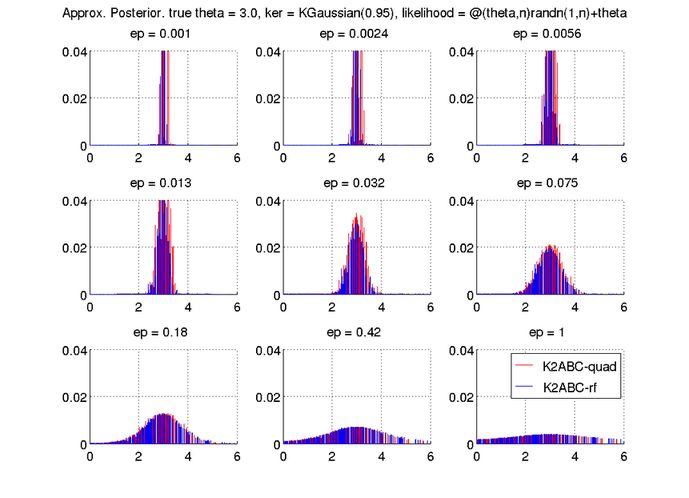
In both K2-ABC with full quadratic MMD (K2ABC-quad), and K2-ABC with
random features (K2ABC-rf), the posterior samples concentrate around the true mean 3.
We observe that small epsilons tend to yield posterior distributions with smaller variance.